Building my first 3D LiDAR odometry: Lessons from the ground up
Have you wonder once, “Well, I have read through so many papers, taken so many courses related to SLAM and localization but somehow I am still not sure how to implement the whole code base myself.”. If you had this thought once during your learning process, then you are not alone, my friend. Today I will share my experience of how I had tackled this dilemma myself after years and years and comprehending how pose estimation and SLAM actually works despite how many literature I had gone throughout all this time.
For now, let’s start simple. My aim is to be able to build up a framework that I can visualize the results of running odometry through a public dataset. I want to lay down the groundwork to be able to run a benchmark, and based on the evaluations to iterate on improvement the current implementation. Hopefully, I can get a pretty a grasp of SLAM by the end of the whole journey.
So, sit back and relax, we are about to begin.
Background
So why do we bother to come up with creating and running an odometry in the first place? To answer this, we have to define what is an odometry. And don’t worry if your text editor consider this a wrongy spelled word because it isn’t. This word is composed of two Greek word - odos meaning “route”, and metron means “measure”. Odometry, therefore, is any type of appraoch to estimate using motion sensors to estimate change in position over time [1]. The most straight forward odometry that you may be first taught at the robotics 101 is to deduce the change in pose of your robot by counting how many wheel spins there were in any given time since the robot set off for a casual stroll. And for legged robots and drones, there are other alternatives to estimate the poses. One of these options is to deduce from the 3D lidar point clouds. Today I want to implement an odometry based on the point clouds. There are three advantages adopting a 3D LiDAR odometry compared to other types of odometry:
- Laser depth readings from a 3D LiDAR are straight-forward in terms of measurements and the point cloud resolution of higher than some of the radar
- 3D LiDAR odometry does not necessarily rely on other motion sensors to estimate the changes in pose, which is convenient to employ for non-wheeled platforms or can contribute to higher pose estimation precision.
- 3D LiDAR sensor can provide a conitnuous stream of point clouds which offer more information of the surrouding than the scans coming from a 2D LiDAR, which in turn only offer a planar surrounding depth reading.
The implementation
I will define the problem and explain how I implement the application to address it.
Define the problem
I once remember that in my first job as a software engineer working to develop the navigation software on an automated guided vehicle (AGV) fleet, the leader of our R&D team once asked the very question: “why can’t we just just count the wheels spins and determine how far the vehicle goes?” Well, this was actually a valid observation if the real-world isn’t that cruel to us. In any real-world scenario, there are discrepancies and uncertainty that comes with the readings from the sensors. For instance, to count the spins that a wheel makes we rely on either mechanical or optical encoders which may yields numbers that are not identical nor crispy all the time, let alone factoring in the discrepancy in readings causing from the wheel friction against the ground. Hence, the farther the vehicle travels, the errors from the encoders add up along time and eventually the deduction of how much distance a vhiecle moved in the space becomes all the less credulous the farther it goes. So the problem boils down to: How to estimate the change of the ego-pose, i.e. the position of the robot in question, by observing the change in the latest observation from the sensor (which is the LiDAR in our case) compared to observation the robot gathered from previous instance(s). Notice that I mentioned from the previous instance(s) and not just a mere previous observation? Because we have the possibility to take into account any previous observation into question to help solve the pose estimtaion problem. And Once we know the poses of the ehicle or robot in question, it is easy to overlap all the observed frames or scans to build a single global map. But what is this map used for? We can use it to determine the vehicle’s position next time when we come around the same area. Hence, we are setting ourselves up to solve the chicken-egg problem of localization and mapping; a sort of catch 22 if you will: In order to know where we are, we need a map; but we can only create a map if we always know where we are.
Here, let me define some key tereminologies to facilitate the coming explanations.
| Terminology | Defnition |
|---|---|
| Frame | The point cloud observed in one single time instance |
| timestamp | The time marked down as either UTC or any arbitrry time |
| Scan | Here will be the synonym of frame |
| Point cloud | A computer science’s abstract data structure to hold multiple spatial coordinates known as points |
| pose | The position of an object, agent, or robot in the space or world |
| ego-pose | Same as pose but emphasizes more on the agent or robot’s point of view |
| state | The position, orientation, and any other attributes you want to include that an agent, vhiecle, or robot holds in a particular instance in time |
Appraoch and methodology
Relying on 3D LiDAR point clouds as the input for an odometry is an interesting task that I am fascinated about. Point cloud per se is a relatively new sensor readings that offer crispier perception of the environment but due to its massive size holding the depth readings, it is also challenging to process the sensor readings known as points and make sense out of them. 3D LiDAR SLAM is still an ongoing esearch topic in robotics and many areas to ccome up with a simple, elegant and efficient algorithm to leverage the massive information that point clouds offer to create a reliable odometry and eventually utterly propose a plausible answer to the SLAM problem.
Let’s talk about the big picture before we dive into the implementation. In my understanding of SLAM and odometry, we can break the pipeline down into the following steps:
-
Input sensor reading pre-processing. This includes denoising, normalizing, downsampling, merging readings from different sensors or tranform the whole inputs under a determined reference frame.
-
In terms of sensor readings as a sequence or stream, we can do a frame-by-frame scan-matching to estimate how much the robot has moved. This is where the core idea of odometry lies.
-
[Optional] Adjust the transitions from one pose to the next in a local fashion, by bundling a couple of frames at a time, such that the estimated poses are more “organic” and accurate to counter the estimation error accumulated as the robot goes along in time.
For each of the mentioned steps, there are a lot of sub-topics and optimization proposition that can be proposed and discussed. But for the scope of this article, we will leave these discussion for later and merely focus on implementing a working pipeline. Although this being said, I still want to lay down the backbone of the pipeline to make it possible to swap in different modules for the mentioned steps to compare how well each proposition is doing. My high-level architectural plan is as follows,
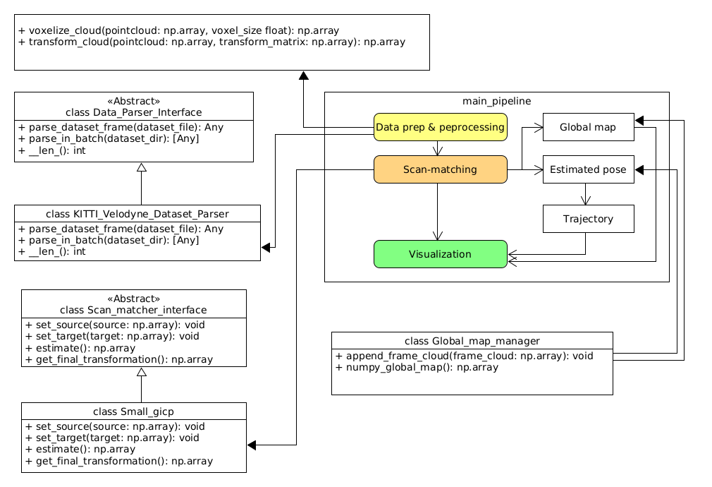 Fig 1. The high-level architecture of the basic odometry
Tools and setups
Since I want to craft a rough prototype to verify that at least my understand works in reality, I will use the following tools:
Programming Language
- Python 3.10+
Modules or libraries
- Numpy (equivalent to Eigen in C++)
- open3d
- small_gicp: We are leveraging the almost real-time efficiency since this project is built on highly optimized multithreaded and GPU lifted C++ codebase
- pangolin: You gotta install and setup python binding module from source. Just follow the instructions on the project’s README.md and you be good.
- other odometry libraries out there, e.g. kiss_icp (GitHub repo)
Coding it up
In this article I have implemented an odometry relying purely on 3D LiDAR point clouds. The dataset used in the following example is the world-famous KITTI Velodyne dataset[2]. The dataset was recorded back in 2012 and is already more than 10 years old however it is still widely used - definitely a good example of being old but gold! A big shout out to the Karlsruhe Institute of Technology team for recording, curating, and releasing these series of benchmark datasets for the whole research and professional communities to use free of charge. Getting back to the odometry, I want to reveal only the key parts of the code snippet while omiting the auxiliary ones. If you want to browse the full code, please visit my repository at basic-slam-pipeline-python - GitHub.
The code is as follows,
import numpy as np
import argparse
from pathlib import Path

# Dataset parsing
from data_processing.data_parser_interface import Data_Parser_Interface
from data_processing.kitti_velodyne_dataset_parser import KITTI_Velodyne_Dataset_Parser

# Scan matching
from scan_matching.scan_matcher_interface import Scan_matcher_interface
from data_processing.coordinate_transformations import voxelize_cloud, transform_cloud
from scan_matching.small_gicp import Small_gicp
from scan_matching.my_gicp import My_GICP
from scan_matching.global_map_manager import Global_map_manager

# visualizers
from visualization.open3d_visualizer import PointCloudVisualizer
from visualization.pangolin_visualizer import Pangolin_visualizer, RED

if __name__=='__main__':
    # (Ommited code)

    # Parse the point clouds
    bin_files = [file for file in dataset_dir.iterdir() if file.suffix == '.bin']
    bin_files = sorted(bin_files)

    print(f'There are in total {len(bin_files)} point cloud files')
    if args.up_to_frame > 0:
        print(f'Running the pipeline up to frame {args.up_to_frame}')
    print('Parsing the dataset...')

    dataset_parser: Data_Parser_Interface = KITTI_Velodyne_Dataset_Parser()
    clouds = []
    if args.up_to_frame > 0:
        clouds = dataset_parser.parse_in_batch(bin_files[:args.up_to_frame])
    else:
        clouds = dataset_parser.parse_in_batch(bin_files)

    print(f'Successfully parsed {len(clouds)} frames')
    print(50 * '-')

    print('Run scan matching...')
    scan_matcher: Scan_matcher_interface = Small_gicp()
    # scan_matcher: Scan_matcher_interface = My_GICP()

    scan_matcher._voxel_size = args.voxel_size

    T_world_lidar = np.identity(4)
    trajectory = [T_world_lidar]
    prev_cloud: np.ndarray = None

    map_manager = Global_map_manager()

    viz = Pangolin_visualizer()

    try:
        for frame_idx, cloud in enumerate(clouds):
            print(f'Processing frame {frame_idx + 1}...')
            voxelized_cloud = voxelize_cloud(cloud[:, :3], args.voxel_size)

            ground_truth_poses = None if args.ground_truth is None else ground_truth_poses

            if frame_idx == 0:
                scan_matcher.set_target(voxelized_cloud)

                # Scan-to-scan
                prev_cloud = voxelized_cloud

                map_manager.append_frame_cloud(voxelized_cloud)

                viz.draw_frame_cloud(pointcloud=voxelized_cloud, trajectory=trajectory, at_idx=frame_idx, gt_poses=ground_truth_poses)

                map_manager.append_frame_cloud(voxelized_cloud)
                continue

            scan_matcher.set_source(voxelized_cloud)
            scan_matcher.set_target(prev_cloud)
            T_world_lidar = scan_matcher.estimate()

            trajectory.append(T_world_lidar)

            frame_cloud = transform_cloud(voxelized_cloud[:, :3], T_world_lidar)

            map_manager.append_frame_cloud(frame_cloud)

            # scan-to-scan
            prev_cloud = voxelized_cloud

            viz.draw_frame_cloud(pointcloud=frame_cloud, trajectory=trajectory, at_idx=frame_idx, gt_poses=ground_truth_poses)

    except Exception as err:
        print(f'Error: {err}')

    # Visualize the global map
    print('Visualizing the global map...')
    viz.hold_on_one_frame(map_manager.numpy_global_map(), trajectory, len(trajectory) - 1, gt_poses=ground_truth_poses)

    # (Ommitted code)

    print('Done')
Let’s break it down.
Data Loading
# Parse the point clouds
bin_files = [file for file in dataset_dir.iterdir() if file.suffix == '.bin']
bin_files = sorted(bin_files)
print(f'There are in total {len(bin_files)} point cloud files')
if args.up_to_frame > 0:
    print(f'Running the pipeline up to frame {args.up_to_frame}')
print('Parsing the dataset...')
dataset_parser: Data_Parser_Interface = KITTI_Velodyne_Dataset_Parser()
clouds = []
if args.up_to_frame > 0:
    clouds = dataset_parser.parse_in_batch(bin_files[:args.up_to_frame])
else:
    clouds = dataset_parser.parse_in_batch(bin_files)
print(f'Successfully parsed {len(clouds)} frames')
This section:
- Collects all binary point cloud files (.bin) from the dataset directory.
- Sorts them to ensure sequential processing
- Creates a parser for the KITTI Velodyne dataset format
- Allows processing a subset of frames with the up_to_frame parameter
- Parses the binary files into point cloud arrays for further processing
Setting up scan-matching and data structures
print('Run scan matching...')
scan_matcher: Scan_matcher_interface = Small_gicp()
# scan_matcher: Scan_matcher_interface = My_GICP()
scan_matcher._voxel_size = args.voxel_size
T_world_lidar = np.identity(4)
trajectory = [T_world_lidar]
prev_cloud: np.ndarray = None
map_manager = Global_map_manager()
viz = Pangolin_visualizer()
Here I initialize the key components for odometry:
- The scan matcher (using Small_gicp implementation, with My_GICP as an alternative option)
- Setting the voxel size parameter for downsampling point clouds
- Creating an identity matrix as the initial transformation (starting pose)
- Initializing an empty trajectory list with the initial pose
- Setting up a map manager to build the global point cloud map
- Creating a visualizer to display results during processing
The main processing loop
try:
    for frame_idx, cloud in enumerate(clouds):
        print(f'Processing frame {frame_idx + 1}...')
        voxelized_cloud = voxelize_cloud(cloud[:, :3], args.voxel_size)
        ground_truth_poses = None if args.ground_truth is None else ground_truth_poses

        if frame_idx == 0:
            scan_matcher.set_target(voxelized_cloud)
            # Scan-to-scan
            prev_cloud = voxelized_cloud
            map_manager.append_frame_cloud(voxelized_cloud)
            viz.draw_frame_cloud(pointcloud=voxelized_cloud, trajectory=trajectory,
                                at_idx=frame_idx, gt_poses=ground_truth_poses)
            map_manager.append_frame_cloud(voxelized_cloud)
            continue

        scan_matcher.set_source(voxelized_cloud)
        scan_matcher.set_target(prev_cloud)
        T_world_lidar = scan_matcher.estimate()
        trajectory.append(T_world_lidar)
        frame_cloud = transform_cloud(voxelized_cloud[:, :3], T_world_lidar)
        map_manager.append_frame_cloud(frame_cloud)
        # scan-to-scan
        prev_cloud = voxelized_cloud
        viz.draw_frame_cloud(pointcloud=frame_cloud, trajectory=trajectory,
                            at_idx=frame_idx, gt_poses=ground_truth_poses)
except Exception as err:
    print(f'Error: {err}')
This is the heart of the odometry system. The convention is to have the take your current frame as the source point cloud (or frame) and the previous frame or the generated map so far as your target. For each frame:
- First frame (frame_idx == 0):
- Set the first cloud as the target for scan matching
- Store it as both the previous cloud and add it to the global map
- Visualize the initial point cloud and trajectory
- That’s it. Move on to the next frame
- Subsequent frames:
- Voxelize (downsample) the current point cloud
- Set up the scan matching between current cloud (source) and previous cloud (target)
- Estimate the transformation matrix (T_world_lidar) using the scan matcher
- Add the new transformation to the trajectory
- Transform the current cloud to the global coordinate system
- Add the transformed cloud to the global map
- Update the previous cloud for the next iteration
- Visualize the current state
The scan-to-scan approach means we’re aligning each new frame with the immediately preceding frame, which is simpler but can accumulate drift over time compared to scan-to-map approaches.
Key technical concepts in this implementation
- Voxelization: Downsampling point clouds to reduce computational load while preserving structural information.
- Scan Matching: Aligning consecutive point clouds to determine the relative motion between frames.
- GICP (Generalized Iterative Closest Point): The algorithm used for scan matching that extends ICP to consider surface normal information.
- Trajectory Estimation: Building a sequence of transformation matrices that represent the vehicle’s path.
- Global Map Building: Accumulating transformed point clouds into a consistent global representation.
Now, let’s dive it to how small_gicp process the state estimation. The following code is the adoption of the example code from the small_gicp repository and is the only approach to works without divergence:
import numpy as np
import small_gicp
from typing import Tuple, Any

from .scan_matcher_interface import Scan_matcher_interface

NUM_THREADS = 7
VOXEL_SIZE = 0.25

class Small_gicp(Scan_matcher_interface):
    def __init__(self):
        self._numThreads: int = NUM_THREADS
        self._voxel_size: float = VOXEL_SIZE

        self._T_last_current: np.ndarray = np.identity(4)
        self._T_world_lidar: np.ndarray = np.identity(4)
        self._target_state: Tuple[np.ndarray, small_gicp.KdTree] = None

    def set_source(self, source: np.ndarray)->None:
        self._source_cloud = source[:, :3]

    def set_target(self, target)->None:
        self._target_cloud = target[:, :3]


    def estimate(self)->np.ndarray:
        downsampled, kd_tree = small_gicp.preprocess_points(self._source_cloud, self._voxel_size, num_threads=self._numThreads)

        if self._target_state is None:
            self._target_state = (downsampled, kd_tree)
            return self._T_world_lidar

        result = small_gicp.align(
            self._target_state[0],
            downsampled,
            self._target_state[1],
            init_T_target_source=self._T_last_current,
            num_threads=self._numThreads
        )

        self._T_last_current = result.T_target_source
        self._T_world_lidar = self._T_world_lidar @ result.T_target_source
        self._target_state = (downsampled, kd_tree)

        return self._T_world_lidar
I want to mention one observation before diving into the code. In my adoption of the small_gicp module as the key odometry algorithm, I’ve tested the raw input point cloud appraoch but the KD tree, as shown in the snippet above, has been the only one that consistently delivers reliable estimamtions throughout the whole dataset. Let me walk you through the code and explains why it works. Let’s focus on the core part:
def estimate(self)->np.ndarray:
    downsampled, kd_tree = small_gicp.preprocess_points(self._source_cloud, self._voxel_size, num_threads=self._numThreads)

    if self._target_state is None:
        self._target_state = (downsampled, kd_tree)
        return self._T_world_lidar

    result = small_gicp.align(
        self._target_state[0],
        downsampled,
        self._target_state[1],
        init_T_target_source=self._T_last_current,
        num_threads=self._numThreads
    )

    self._T_last_current = result.T_target_source
    self._T_world_lidar = self._T_world_lidar @ result.T_target_source
    self._target_state = (downsampled, kd_tree)

    return self._T_world_lidar
This is where the magic happens. Let’s break it down:
- Preprocessing the source cloud:
downsampled, kd_tree = small_gicp.preprocess_points(self._source_cloud, self._voxel_size, num_threads=self._numThreads)
The current frame or point cloud is downsampled with the specified resolution voxel_size. Downsampling the incoming point cloud reduces computation load. The input cloud is also saved in a KD tree which helps in correspondence matching later on.
- Handling the first frame
if self._target_state is None:
    self._target_state = (downsampled, kd_tree)
    return self._T_world_lidar
For the first frame, there is no previous cloud to align with, so I simply cache the preprocessed cloud and its KD-tree while returning the initiaal pose, in this case is the world’s origin expressed as an identity matrix.
- Aligning point clouds
result = small_gicp.align(
    self._target_state[0],
    downsampled,
    self._target_state[1],
    init_T_target_source=self._T_last_current,
    num_threads=self._numThreads
)
This is actally a wrapper function to the related C++ function. The align function used here is one of polymorphic functions that take in this particular set of arguments:
- target cloud
- source cloud
- the source KD-tree
- initial guess as a 4x4 transformation matrix
- number of threads for parallel computation
So, I pass in the following:
- The cached target (previous) point cloud
- The downsampled source (current) point cloud
- The KD-tree from the target point cloud for efficient correspondence finding
- The previous transformation as an initial guess to warm-start the alignment
- number of threads
- Updating transformation
self._T_last_current = result.T_target_source
self._T_world_lidar = self._T_world_lidar @ result.T_target_source
I store the relative transformation for use as the initial guess in the next frame, and update the cumulative world transformation by matrix multiplication.
- Preparing for next frame
self._target_state = (downsampled, kd_tree)
I update the cached target state with the current cloud to use it as the target in the next iteration.
Why does this implementation works so well?
This implementation of odometry on GICP using KD-tree has proven to be an efficient method in my testing for several reasons:
-
Efficient data structures: As all tree in computer science, the data structure enables $O(\log n)$ nearest neighbor searches rather than $O(n)$ brute force comparison, making real-time processing possible even with dense point clouds.
-
Voxel downsampling: Reducing the point cloud density through oxelization preserves structural information while dramatically reducing computation time.
-
Multi-threading: Utilizing parallel processing for both preprocessing (downsampling and KD-tree construction) and alignemnt accelerates the most computationally intensive operations.
-
Warn starting: Using the previosu transformation as an intial guess significantly speeds up convergence and improves robustness when vehicle motion is relatively smooth.
-
Transformation composition: Properly composing transformation maintains a consistent global reference frame throughout that trajectory.
I had tried with other alignment approaches that caused me no short of headache on the great number of parameters to fine-tune, the dissapointing low number of inliers after certain frame, or ever inceasing error with more inbound frames. In contrast, this setup of having GICP working with KD-tree strikes a decent balance between computation speed and accuracy, making it viable for real-time odometry as we have discussed so far.
Challenges faced
I only want to limit my discussion on the implementation and testing aspects of this application. There is always a tradeoff bewteen keeping the number of frame-wise points low and manageable enough to take care of the computation efficiency while also have enough points to do a meaningful frame-to-frame or map-to-frame alignment. I picked the voxel size of 0.5 to be a reasonable number to balance both factors.
And inevitably with the mentioned constraints, the odometry can get as good as it can get with a catch: there is more notieable of a position drifting the longer the vehicle moves. An assistance is needed to “fix” the traversed trajectory locally to…put the right poses back to their places. To achieve so, there are a couple of maneuvres at our disposal, such as involve a second sensor (an IMU, GPS or camera) reading as an extra source of reference to do the correction via Bayesian filtering, or consider registering the estimated poses in a pose graph and do some local and global bundle adjustments to refine the trajectories and estimated poses.
Additionally, tere are around 5 occasions in the dataset that a loop closure can be detected and taken advantage of to refine the trajectory. If the loop closure is applied, the overall pose estimation would be greatly improved.
Results
Despite of the points I mentioned in the section “Challenges found”, the result is aleady quite impressive that by just running the scan-matching on a frame-by-frame basis the estimated poses and the rendered map are already reasonably aligned and correct. For the actual result, please refer to Figure 2.
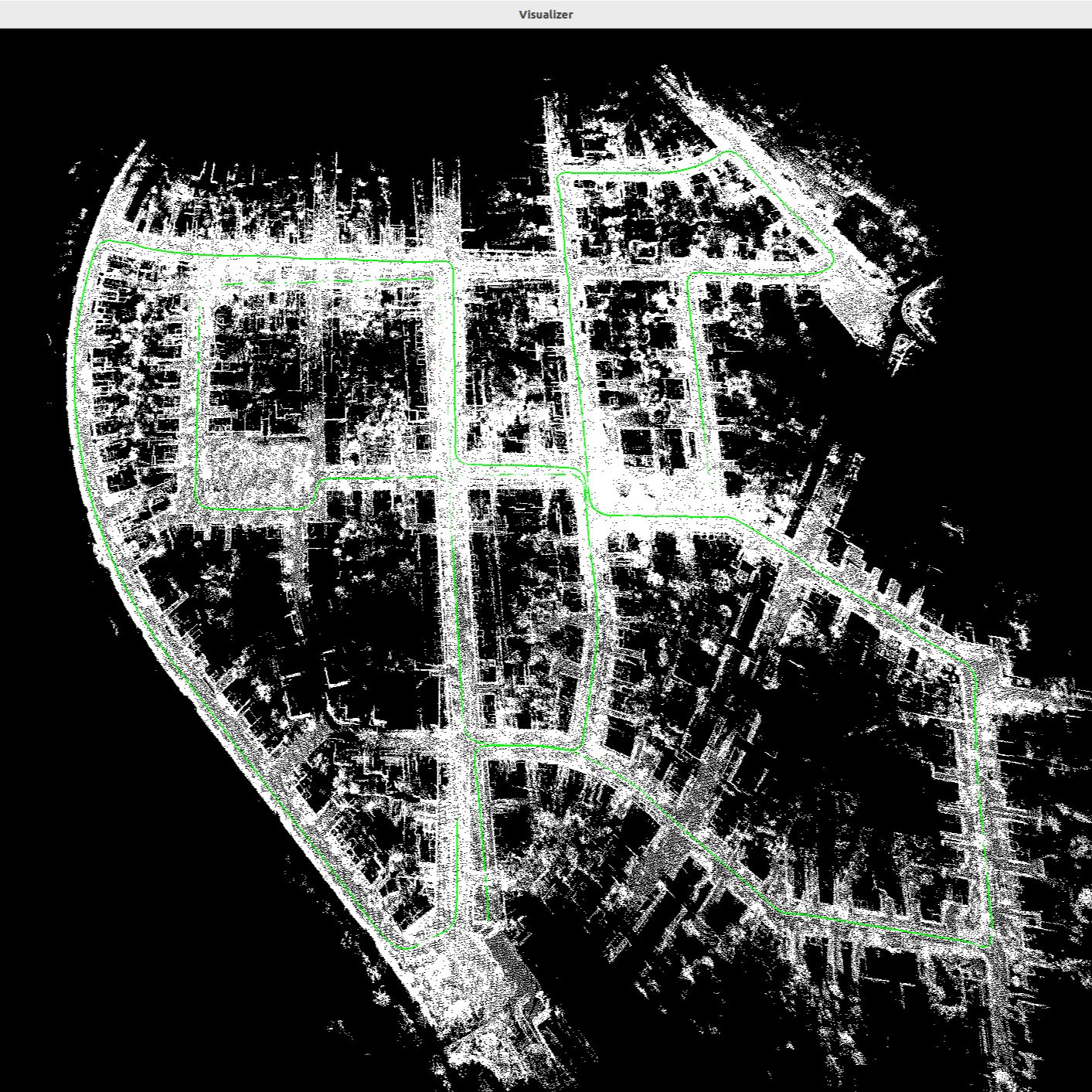 Figure 2. The KITTI Velodyne dataset recorded on various streets at the city of Karlsruhe. The estimated trajectory and the global map are drawn directly with the result of the odometry estimation alone.
There will be a demo video coming up soon.
Lessons learned
The practicality of designing and implementing an odometry factors in the available sensors and the quality of the gathered sensor data, what are the physical limitations of the sensor (I can go on for another hour on 3D LiDAR. No worries. Article coming soon), the tradeoff between achieving real-time computation efficiency vs the required accuracy on the estimated poses, and how much computation power can a platform provide. In addition, we can also consider whether it is viable to do a sensor fusion to increase the estimation accuracy or to optimize the algorithm based on actual business needs to fine-tune the odometry and SLAM pipeline to achieve the best performance under the existing physical and computational constraints.
Next steps
This is just the beginning. As mention at the beginning of the article, there are several steps to take in order to make it into a formidable SLAM application:
- Odometry (Done but can keep trying other appraocches)
- Introduce ground truth and benchmark with RMSE and other metrics
- (local and global) Pose optimization
- Implement Loop closure
- Port the code to C++
- Scale up the code to take on different datasets
- Run performance profiling to pin-point and eliminate bottle-neck
Conclusion
This article presents my implementation of a basic odometry that sereves as future foundation for a SLAM pipeline. Apart from walking through the different parts of the odometry, I also discussed the challenges and propositions to improve the current performance of the odometry. Hopefully this article helps you in your implementation or engages your curiousity and passion about this area of robotics.
References
- [1] Odometry - Wikipedia
- [2] Geiger, Andreas, Philip Lenz, and Raquel Urtasun. “Are we ready for autonomous driving? the kitti vision benchmark suite.” 2012 IEEE conference on computer vision and pattern recognition. IEEE, 2012.